This lesson explores the fundamental concepts of histograms, their construction, and interpretation, essential for representing grouped continuous data.

CAIE A-level S1 Syllabus

• draw and interpret histograms

What is a Histogram?

A histogram serves as a graphical representation primarily used for visualizing grouped continuous data. While it shares visual similarities with a bar chart, crucial distinctions exist:

• Data Type: Histograms are specifically designed for continuous data that has been grouped into classes, whereas bar charts are suitable for discrete or qualitative (categorical) data.
• Bar Adjacency: A defining characteristic of histograms is the absence of gaps between adjacent bars, signifying the continuous nature of the data range they represent.
• Vertical Axis Scale: In a bar chart, the height of a bar directly indicates the frequency. However, in a histogram, the height of each bar represents frequency density.

Plotting frequency density on the y-axis is particularly advantageous when dealing with unequal class intervals, as it accurately reflects the distribution of data, especially when values are spread unevenly at the ends of the range.

Importantly, the area of each bar within a histogram is directly proportional to the frequency of observations within that specific class interval.

Constructing a Histogram

Follow these methodical steps to accurately draw a histogram:

• Step 1: Address Class Interval Gaps. Before any calculations, meticulously inspect the data for any gaps between the upper boundary of one class and the lower boundary of the subsequent class. If such gaps exist, they must be closed. This involves adjusting the boundaries; consider whether the original data values were rounded or truncated when making these adjustments.
• Step 2: Determine Class Widths. For each group, calculate the class width by subtracting its lower boundary from its upper boundary.
• Step 3: Calculate Frequency Density. Compute the frequency density for every group using the following formula:
  \text{Frequency density} = \frac{\text{Frequency}}{\text{Class Width}}
• Step 4: Plot the Histogram. Draw the histogram with the data values positioned along the x-axis and the calculated frequency density on the y-axis. Remember these key plotting guidelines:
  • Ensure that the scale on both axes is consistent, even if the class widths themselves are not uniform.
  • Both axes should be clearly labeled, and units should be included for the x-axis, which represents the data values.
  • Due to potentially varying class widths, the bars will often have different widths.

Interpreting a Histogram

Correct interpretation of a histogram requires understanding that the y-axis does not directly show frequency.

• The frequency for a given class is found by multiplying its frequency density by its class width:
  \text{Frequency} = \text{Frequency Density} \times \text{Class Width}
• If asked to determine the frequency of a segment of a bar within a histogram, calculate the area of that specific segment using the frequency density and the corresponding part of the class width.

Worked Example

The table below presents data on the lengths, in cm, of a sample of freshly picked green beans, alongside its corresponding histogram.

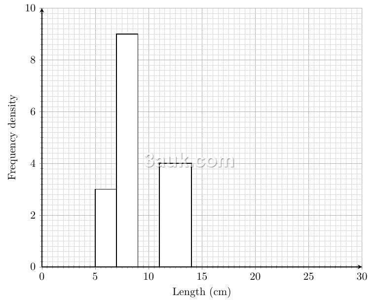
(a) Complete the histogram.

(b) Estimate the number of green beans whose length is greater than 12 cm.

Answer:

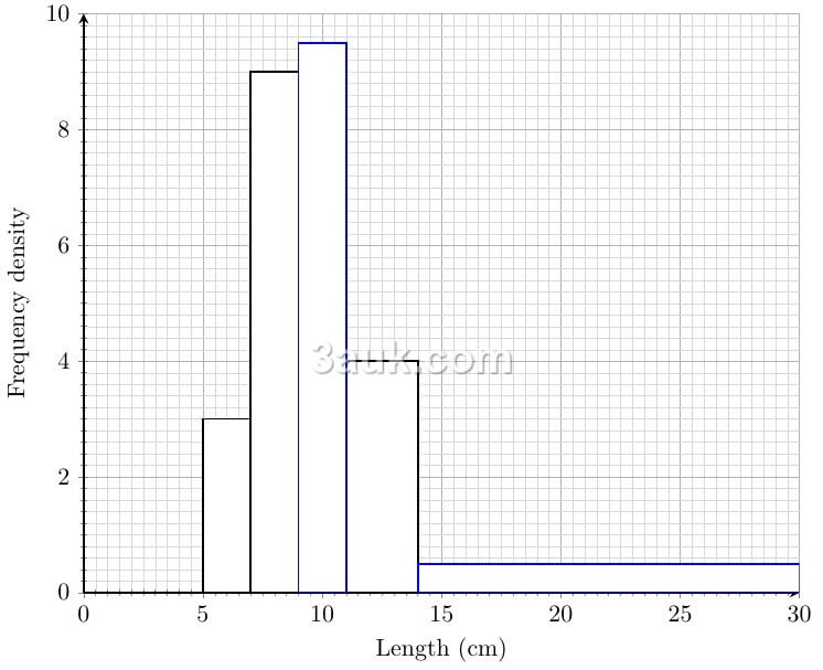
(a) First, calculate the frequency density for the classes 9 \leq L < 11 and 14 \leq L < 30.

\text{Frequency density} = \frac{\text{Frequency}}{\text{Class Width}}

For 9 \leq L < 11:

FD = \frac{19}{2} = 9.5

For 14 \leq L < 29:

FD = \frac{8}{16} = 0.5

Now, draw the bars on the provided histogram diagram using these calculated frequency densities.

(ii) To estimate the number of green beans with a length greater than 12 cm, we need to consider two parts:

• The portion of the 11 \leq L < 14 class that is greater than 12 cm (i.e., 12 \lt L < 14).
• The entire 14 \leq L < 30 class.

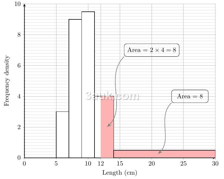
For the class 11 \leq L < 14:

• Class width = 14 - 11 = 3
• Frequency = 12
• Frequency density = 4

For the interval 12 \lt L < 14:

• Width = 14 - 12 = 2
• Estimated frequency = \text{Frequency Density} \times \text{Width} = 4 \times 2 = 8 green beans

For the class 14 \leq L < 30:

• Frequency = 8 green beans

Total estimated number of green beans greater than 12 cm = 8 + 8 = 16.

An estimated 16 green beans have a length greater than 12 cm.

Examiner Guidance

Always pay close attention to the scales provided on both axes of a histogram. They are rarely simple one-unit-per-square increments. Misinterpreting the scale can lead to significant errors in calculations and interpretations.