Ever wondered why producing more steak could lead to cheaper leather boots? Dive into the fascinating concept of joint supply in economics, a key topic for A-Level students that explains how goods are produced together, impacting markets in unexpected ways. This isn’t just theory—it’s the reason behind fluctuating prices in agriculture and energy sectors. Get ready to unravel how joint supply makes economics relatable and essential for understanding real-world markets. For a solid foundation in CAIE A-Level Economics, check out our beginner-friendly starter guide to build on these interconnected ideas.
Understanding Joint Supply in Economics
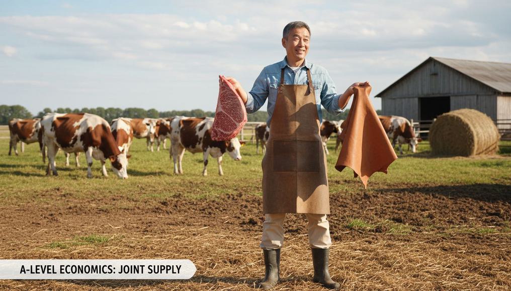
Joint supply occurs when two or more products emerge simultaneously from the same production process, much like uninvited guests at a party. Imagine raising cattle primarily for beef, the star product that drives your farm’s profits. But along comes leather as the joint product, a byproduct you can’t avoid. In A-Level economics, this concept highlights how increasing output for one good inevitably boosts supply for the other, often leading to price shifts.
The primary product, like beef, is what producers aim for, while the joint product, such as leather, follows suit. When demand for beef surges—think the global protein boom—farmers ramp up production. This floods the leather market too, potentially driving down leather prices if demand doesn’t keep pace. For beginners in A-Level economics, this builds on basic supply and demand principles but adds a layer of interconnectedness that’s crucial for exams. To deepen your grasp of these fundamentals, explore our guide to the price system and microeconomy.
Real-life disruptions, like the 2022 Ukraine conflict, slashed wheat production by 41%, affecting not just grain but also straw used for animal bedding [UkrAgroConsult, 2023]. This shows how joint supply creates ripples across industries. Ignoring it is like overlooking plot twists in your favorite series—you’ll miss the full story, especially when tackling A-Level data response questions.
Real-World Examples of Joint Supply
Theory comes alive through current events, making joint supply in economics more than abstract graphs. In agriculture, wheat and straw exemplify this: Farmers grow wheat for food staples, but the stalks become straw for livestock or biofuels. During the Ukraine crisis, wheat output dropped to 19.5 million metric tons, dragging straw supply down and spiking prices for both [USDA, 2024]. By 2023, recovery to 23.4 million tons stabilized markets, illustrating the tight link. These scenarios tie into broader production concepts, like those covered in our guide to production possibility curves, helping you see resource trade-offs in action.
Beef and leather provide a classic A-Level economics case. U.S. beef production reached 12 million metric tons in 2023, fueled by post-pandemic demand [USDA, 2023]. As Asian markets craved more beef, cattle numbers rose, surging leather supply and causing an 8% price drop in 2022. Producers faced a surplus of hides while celebrating meat sales—a perfect example of joint supply dynamics.
Sheep farming in New Zealand tells a similar tale, with 25-30 million sheep yielding mutton and wool jointly [Statistics New Zealand, 2023]. A decline in flock sizes increased prices for both by 10%, impacting exports. Beyond farms, oil refining produces petrol and butane together. With global oil at 103 million barrels daily in 2023, excess refining for fuel led to a 10-15% butane price fall during supply gluts [IEA, 2023]. Flour milling follows suit: U.S. output of 140 million tons in 2023 kept bran, used in feeds and compost, affordably steady [USDA, 2023]. These cases, tied to $3 trillion in agricultural trade, underscore why mastering joint supply is vital for A-Level success [World Bank, 2023].

Illustrating Joint Supply with Diagrams
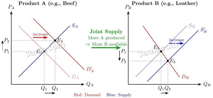
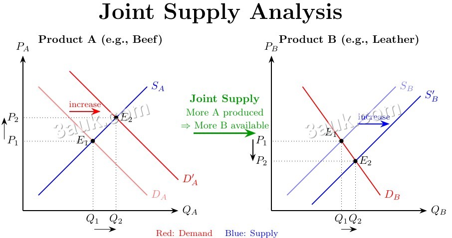
Visuals are your best friend in A-Level economics, turning complex ideas like joint supply into exam gold. Start with two adjacent graphs: one for the primary product (beef) and one for the joint (leather).
1. On the beef graph, demand curve DA meets supply SA at equilibrium E1 (price P1, quantity Q1). A demand increase to DA‘ shifts equilibrium to E2, raising price to P2 and quantity to Q2.
2. For leather, initial supply SB intersects demand DB at E1 (P1, Q1). The beef production boost shifts leather’s supply right to SB‘, creating new equilibrium E2 with higher quantity Q2 but lower price P2. This spillover effect is the heart of joint supply in economics—one market’s gain can pressure another’s prices.
3. To summarize, when demand for Product A increases, producers supply more A. This automatically increases supply of B, lowering B’s price (assuming B’s demand remains constant).
The key insight: When two products are jointly supplied (like beef and leather from cattle), an increase in demand for one product leads to increased production of both products. This causes the price of the joint product to fall due to increased supply, assuming its demand remains constant.
Assumptions simplify: Fixed production ratios and constant joint demand. In practice, Brazil’s 2020s beef expansion increased leather volume by 15% but lowered prices 8% [FAO, 2023]. For exams, label shifts clearly and explain: ‘Rising beef demand enhances joint leather supply, reducing its price.’ Reverse scenarios, like falling demand, show price rises for both. Link to policies, such as subsidies for byproducts, to deepen analysis and ace essays.

Joint Supply Versus Joint Demand
Don’t confuse joint supply with joint demand—they’re related but distinct in A-Level economics. Joint supply is production-focused: Goods like beef and leather arise together, so supply changes in one affect the other directly, without much elasticity involvement.
Joint demand, however, involves complementary goods consumers buy together, like printers and ink. A price drop in ink boosts printer demand due to negative cross-price elasticity (e.g., 10% ink reduction lifts printer sales 5-7%). Examples include razors and blades or cars and petrol pre-electric vehicles. For more on how price changes influence demand, dive into our beginner’s guide to price elasticity of demand.
Compare them:
| Aspect | Joint Supply | Joint Demand |
|---|---|---|
| Focus | Production from shared source | Consumer complementarity |
| Examples | Beef & leather; oil & butane | Printers & ink; cars & petrol |
| Impact | Supply shift in one affects the other | Price change in one influences demand for the other |
| Elasticity | Primarily supply-side | Negative cross-price elasticity |
Emerging trends, like biofuels from straw, merge these concepts in sustainable economies [EU Eurostat, 2024]. For A-Levels, remember: Supply ties producers, demand ties buyers.

Practical Tips and FAQs for A-Level Success
Apply joint supply knowledge to excel:
- Diagram Practice: Weekly sketches of beef-leather scenarios; use online tools for precision. Supplement with our CAIE AS Level Economics study notes for visual aids.
- News Integration: Track wheat prices and connect to straw impacts in current events for essay depth.
- Comparisons: Quiz on supply vs. demand differences, like oil gluts affecting fuels but not vehicles. Test yourself with CAIE A2 Economics topic questions for targeted practice.
- Policy Insights: Explore how EU biofuel incentives valorize byproducts [EU Eurostat, 2024].
- Exam Strategies: Assume stable joint demand; reference sectors like agriculture or energy in responses.
FAQs:
1. Primary vs. joint products? Primary drives production (beef); joint is secondary (leather), but both influence prices.
2. Price effects? Primary demand rise increases its price, often lowers joint’s via excess supply.
3. Avoidable? No, inherent to processes; technology may adjust ratios slightly.
4. Non-ag example? Natural gas yields oil as joint product, linking energy markets.
5. Diagram advice? Side-by-side graphs with shifts; arrows ensure clarity.
6. Elasticity role? Minimal in supply; save for demand’s complements.
7. A-Level relevance? Key for intermarket questions, like Ukraine’s ag disruptions.
8. Trends? Sustainable uses, e.g., cotton byproducts in biofuels [World Bank, 2023].
Grasp joint supply in economics, and you’ll navigate A-Level challenges effortlessly, predicting market twists like a pro.
References
- Joint Supply. Retrieved from https://www.economicshelp.org/blog/glossary/joint-supply/
- UkrAgroConsult. (2023). Ukraine Grain Production Estimates. Retrieved from https://www.ukragroconsult.com/
- USDA Foreign Agricultural Service. (2024). Wheat Production Data. Retrieved from https://www.fas.usda.gov/data
- USDA. (2023). Beef and Flour Production Reports. Retrieved from https://www.usda.gov/topics/farming
- IEA. (2023). World Energy Outlook. Retrieved from https://www.iea.org/reports/world-energy-outlook-2023
- Statistics New Zealand. (2023). Sheep Farming Report. Retrieved from https://www.stats.govt.nz/
- FAO. (2023). Leather Market Analysis. Retrieved from https://www.fao.org/home/en/
- World Bank. (2023). Agricultural Trade Overview. Retrieved from https://www.worldbank.org/en/topic/agriculture
- EU Eurostat. (2024). Biofuel Policies and Crop Byproducts. Retrieved from https://ec.europa.eu/eurostat